Least Squares Regression as an Orthogonal Projection
In my adventures through Mathematics for Machine Learning, I discovered that linear regression can actually be interpreted geometrically as an orthogonal projection - and this blew my mind. As a firm believer that any concept becomes much more interesting with the addition of cute, fluffy animals, here I’m going to illustrate this concept with some (imaginary) sheep.
We have 5 sheep and we know the weight of wool each sheep produced last year. All 5 of our sheep produced very different amounts of wool! We want to know what factors cause this variation between sheep, so we decide to measure some variables: food intake, water intake, and average hours of sleep per day.
> wool <- c(10, 20, 30, 40, 50)
> grass <- c(25.2, 60.4, 82.5, 100.1, 120)
> water <- c(40.2, 21.5, 28.8, 68, 21)
> sleep <- c(8, 6, 2.5, 1.1, 1.1)
> sheep <- data.frame(wool, grass, water, sleep)
Now we will reframe our data frame as a regression equation.
$$ \begin{equation} \mathbf{y = Xb + e} \end{equation} $$Where $\mathbf{y}$ is a (5 x 1) vector of wool measurements, $\mathbf{X}$ is a (3 x 5) design matrix that relates each wool measurement to the corresponding water, grass, and sleep measurements, $\mathbf{b}$ is a (3 x 1) vector of regression coefficients for the variables water, grass, and sleep, and $\mathbf{e}$ is a (5 x 1) vector of residual errors. Below I rename the R variables according to their names in the above equation, so you can see how the collected data are involved in the regression.
> X <- as.matrix(sheep[,2:4])
> y <- wool
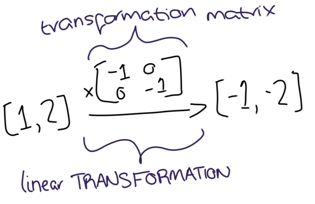
Projections are a special class of linear transformation: they map on vectors on one plane onto vectors on another plane. Mathematically, such transformations can be represented by transformation matrices which apply the linear transformation to the vector. Transformation matrices for projections, called projection matrices ($\mathbf{P}$) always follow $\mathbf{P^2 = P}$.

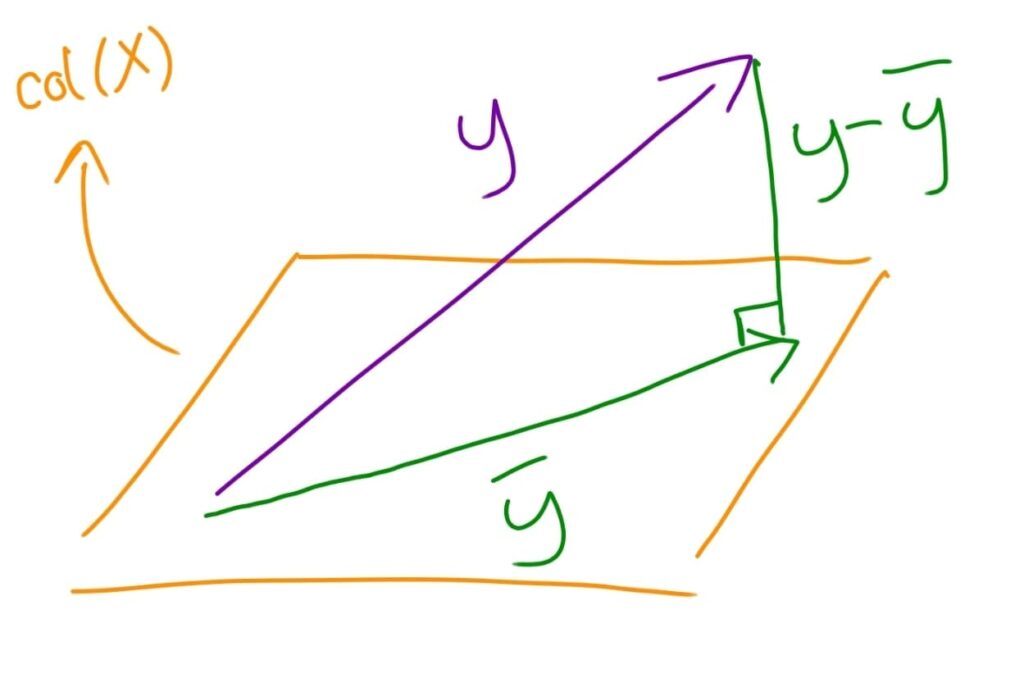
Essentially, regression performs an orthogonal projection of $\mathbf{y}$ onto the column space of $\mathbf{X}$. To picture this, we’d need to “imagine” a 5-dimensional space containing the vector $\mathbf{y}$. There is also a plane, defined by the column space of $\mathbf{X}$ (i.e. a plane encompassing all possible linear combinations of the vectors for grass, water, and sleep). In an orthogonal projection, the transformation finds the vector in the plane being projected to (in this case, the column space of $\mathbf{X}$) that is closest to the original vector (in this case, $\mathbf{y}$). I will call this vector $\mathbf{\hat{y}}$, for reasons that will become apparent later. This will always occur when the vector that joins $\mathbf{y}$ to its projection in $\mathbf{X}$ (which I will refer to as $\mathbf{y - \hat{y}}$) is at right angles to the column space of $\mathbf{X}$.

So essentially, we are finding how the wool data best fits onto the grass, water, and sleep data. Let’s return to our data for a mathematical example. First, to find the projection matrix for transforming vectors into the column space of $\mathbf{X}$ we use:
$$ \begin{equation} \mathbf{P = X(X^TX)^{-1}X^T} \end{equation} $$> P <- X %*% solve(t(X) %*% X) %*% t(X)
We can prove this is a projection matrix because $\mathbf{P^2 = P}$:
> P
            [,1]       [,2]       [,3]        [,4]        [,5]
[1,]  0.73792943  0.3549499 0.04904521  0.09499315 -0.23658199
[2,]  0.35494988  0.4419646 0.18057488 -0.18219850  0.23417705
[3,]  0.04904521  0.1805749 0.20144971  0.15332376  0.31991690
[4,]  0.09499315 -0.1821985 0.15332376  0.92848041  0.02600719
[5,] -0.23658199  0.2341770 0.31991690  0.02600719  0.69017591

> P %*% P
            [,1]       [,2]       [,3]        [,4]        [,5]
[1,]  0.73792943  0.3549499 0.04904521  0.09499315 -0.23658199
[2,]  0.35494988  0.4419646 0.18057488 -0.18219850  0.23417705
[3,]  0.04904521  0.1805749 0.20144971  0.15332376  0.31991690
[4,]  0.09499315 -0.1821985 0.15332376  0.92848041  0.02600719
[5,] -0.23658199  0.2341770 0.31991690  0.02600719  0.69017591
As this is the projection matrix for the column space of $\mathbf{X}$, we know that the vector grass lies on this plane. Thus, if we try to apply the projection matrix onto grass, we should just get grass. Indeed, this is exactly what we see!
> grass
[1]  25.2  60.4  82.5 100.1 120.0

> grass %*% P
     [,1] [,2] [,3]  [,4] [,5]
[1,] 25.2 60.4 82.5 100.1  120
So now we have the projection matrix for the column space of $\mathbf{X}$, let’s project $\mathbf{y}$ onto the column space of $\mathbf{X}$!
> y %*% P
         [,1]     [,2]     [,3]     [,4]     [,5]
[1,] 7.920275 22.22695 32.27424 40.34525 47.46431

> model <- lm(wool ~ grass + sleep + water)
> model\$fitted.values
        1         2         3         4         5
 7.926969 22.814584 30.366039 40.756166 48.136242
Note that this vector is very close to the fitted values of the regression model, but unfortunately they are not exactly identical in my example because of rounding errors resulting from computation with floating point numbers. Nevertheless, mathematically, the projection of $\mathbf{y}$ on the column space of $\mathbf{X}$ gives the vector $\mathbf{\hat{y}}$ which is a vector of the fitted values. That is, the best wool estimates for our five sheep given their grass intake, water intake, and sleeping habits.
The residuals are the difference between the fitted values and the true wool values for the sheep. If our geometric interpretation is correct, these should represent the vector $\mathbf{y - \hat{y}}$. If so, it is orthogonal to the column space of $\mathbf{X}$, and thus the product of $\mathbf{y - \hat{y}}$ and the projection matrix $\mathbf{P}$ should be the zero vector.
> model\$residuals
         1          2          3          4          5
 2.0730312 -2.8145839 -0.3660388 -0.7561661  1.8637575
> P %*% model\$residuals
              [,1]
[1,] -2.220446e-16
[2,] -2.775558e-16
[3,] -2.220446e-16
[4,] -4.579670e-16
[5,] -6.661338e-16
Rounding error means we observe values very close to 0, but not exactly 0. Ignoring the error, we can say that the residuals, $\mathbf{y - \hat{y}}$, are orthogonal to the column space of $\mathbf{X}$, as we would expect if regression was an orthogonal projection of $\mathbf{y}$ onto the column space of $\mathbf{X}$.
What about our regression coefficients, $\mathbf{b}$? These are what actually tell us how strongly each of the factors affect the sheep’s wool production. They are found using the equation:
$$ \begin{equation} \mathbf{b = (X^TX)^{-1}X^T(y} - intercept) \end{equation} $$> model
Call:
lm(formula = wool ~ grass + sleep + water)
Coefficients:
(Intercept) grass sleep water
-19.94155 0.54170 1.41374 0.07233
> solve(t(x) %*% x) %*% t(x) %*% (y + 19.94155)
[,1]
grass 0.54170
water 0.07233
sleep 1.41374
I find this geometric representation of finding the ’least squares’ solution very satisfying. In stats class, you are typically shown how minimising the squared distance between data points and the regression line leads to regression solutions, but I think this is more difficult to imagine than the orthogonal projection when we generalise to more than one predictor.

References
Deisenroth, M. P.; Faisal, A. A.; & Ong, C. S. 2020, Mathematics for Machine Learning, Cambridge University Press.
These videos were also very useful: https://www.youtube.com/watch?v=My51wdv2Uz0