Many Ways to Test a Hypothesis

Trading mathematical rigour for easily revisited intuition, here I describe a number of hypothesis tests in a “refresher friendly” manner. Namely: the Wald test, the likelihood ratio test, and the score test. This post assumes prior understanding of likelihood. As an example, I will take the case of testing the significance of a regression coefficient. Imagine that we have performed a regression analysis to try and find out if sheep growth changes with grass intake:

$$ \begin{equation} \mathbf{y} = \beta_0 + \mathbf{\beta x + e} \end{equation} $$

Where $\mathbf{y}$ is a ($n$ x 1) vector of sheep growth measurements from $n$ randomly sampled sheep; $\beta_0$ is the intercept; $\mathbf{\beta}}$ is the fixed effect of grass intake; $\mathbf{x}$ is the ($n$ x 1) vector of grass intake measurements; and $\mathbf{e}$ is the ($n$ x 1) vector of residual effects.

Assuming that we already have a maximum likelihood estimate (MLE) for $\mathbf{\beta}$, $\mathbf{\hat{\beta}}$, we want to test the null hypothesis that grass intake has no effect on sheep growth: $\mathbf{\hat{\beta}} = 0$. So, how do we go about it?

Wald Test

One way to test this hypothesis would be to use a Wald test. The test statistic, $Q_{Wald}$, for a Wald test is given by:

$$ \begin{equation} Q_{Wald} = \frac{(\hat{\beta} - \beta_{null})^2}{var(\hat{\beta})} \end{equation} $$ $$ \begin{equation} var(\hat{\beta}) = I(\hat{\beta})^{-1} \end{equation} $$

Where $\beta_{null}$ is the expected value of $\beta$ under the null hypothesis. In our example, this is zero. Under the null hypothesis, $Q_{Wald}$ follows asymptotically a $\chi^2$ distribution with 1 degree of freedom. This fact can be shown mathematically (see here if you’re interested in the proof).

What does it actually mean for $Q_{Wald}$ to follow asymptotically a $\chi^2$ distribution with 1 degree of freedom? It means that if we were, for example, to perform our sheep experiment 5000 times randomly sampling a population of sheep whose weight we knew was not influenced by grass intake (“under the null hypothesis”), and then a histogram of all of the $Q_{Wald}$ statistics from all of those experiments would look something like this:

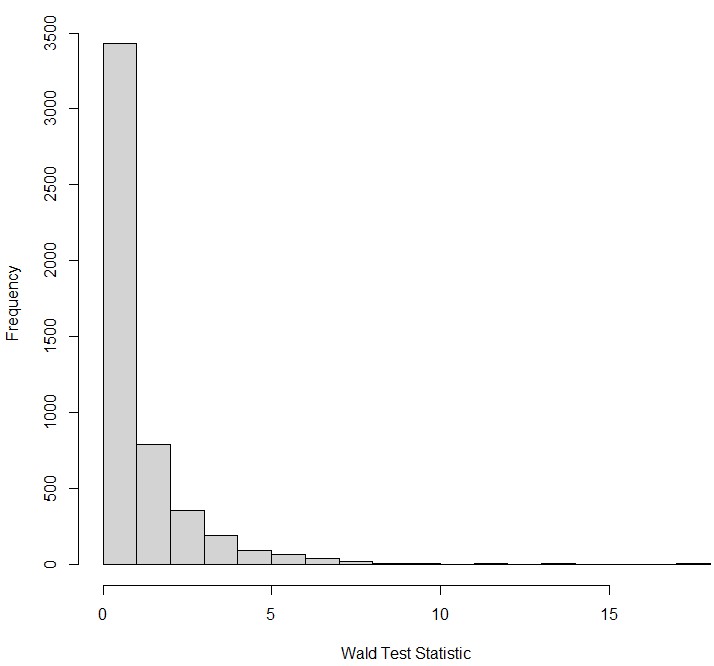
The test statistic varies even though the null hypothesis is true because of sampling error. Notice how this looks similar to the $\chi^2$ distribution with 1 degree of freedom:

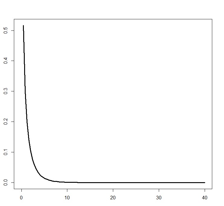Chi square distribution with 1 degree of freedom

As the number of experiments we run under the null hypothesis increases, this histogram approximates the above graph. “Asymptotically” refers to this property: that the more samples you have, the closer and closer to this distribution you are. This is what allows us to use such test statistics to test a hypothesis. Using the $\chi^2$ distribution, we can obtain the probability of obtaining the observed $Q_{Wald}$, or an even more extreme value of $Q_{Wald}$, given that the null hypothesis is true by measuring the area under the $\chi^2$ distribution to the right of this value of $Q_{Wald}$. This probability is the p-value. If this probability is small, then it is less likely that the test statistic was generated from data under the null hypothesis, and we choose instead to accept the alternative hypothesis.

But how exactly, did we get the formula for $Q_{Wald}$? Let’s revisit the formula. Note the numerator: as the difference between $\hat{\beta}$ and $\beta_{null}$ grows, so does $Q_{Wald}$. This makes intuitive sense: a larger $Q_{Wald}$ means a smaller p-value, which means we are more likely to reject the null hypothesis when the estimated effect size is very different to that expected under the null hypothesis.

$$ \begin{equation} Q_{Wald} = \frac{(\hat{\beta} - \beta_{null})^2}{var(\hat{\beta})} \end{equation} $$

This difference is divided by the variance of the maximum likelihood parameter estimate. A visual is useful for understanding why this is the case. Below is a graph of a likelihood function (the solid black line). On the y-axis is the likelihood of the observed data given some parameter value, and the x-axis is different parameter values. The red dashed line represents the MLE of the parameter, and the black dashed line represents the parameter value under the null hypothesis:

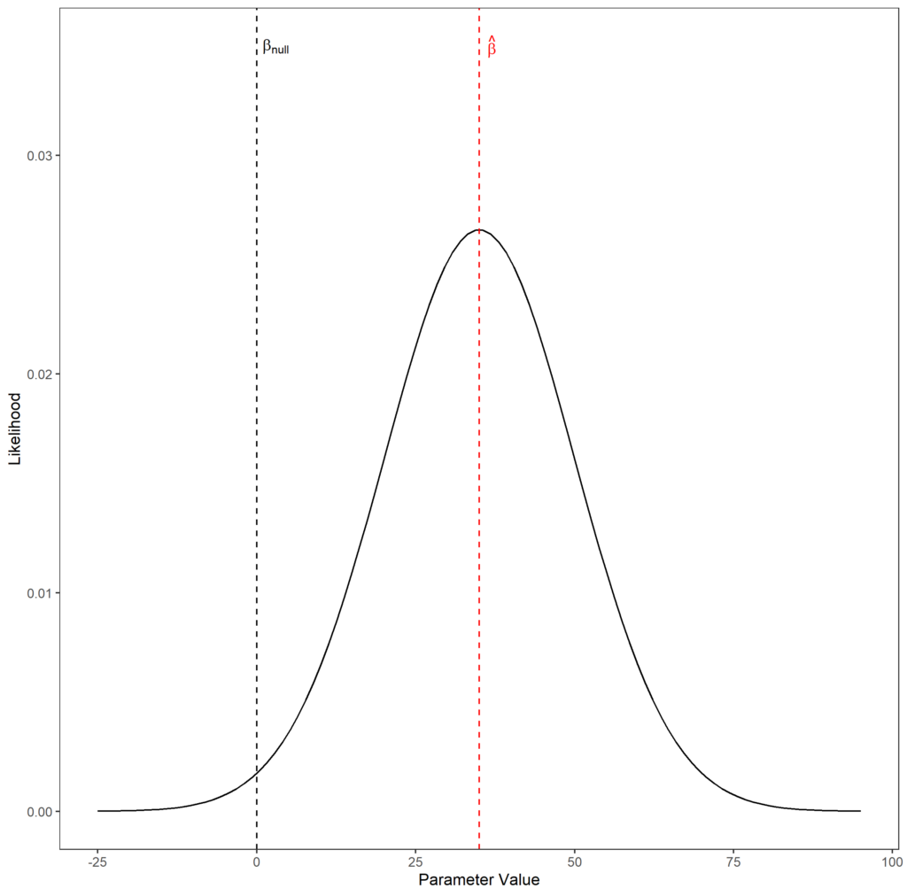
Imagine that the likelihood function is flattened out, but maintained the same maximum likelihood. This would increase the likelihood of the observed data given that the true parameter value was $\beta_{null}$. Likewise, if the likelihood function were narrower than is shown, then the likelihood of the observed data given that the true parameter value is $\beta_{null}$ is reduced. We account for this in the denominator. Here’s why.

Imagine we sample our population of sheep many, many times and for each sample we calculate the MLE $\hat{\beta}$. The true value of $\beta$ is the same in every sample, but sampling error means that $\hat{\beta}$ will differ from sample to sample, thus this parameter has a variance related to this error. If the sampling error is large, a sample of size $n$ gives us less information about the parameter value than a sample of size $n$ from a population with a lower sampling error. Thus, the likelihood function will be flatter, because for every possible parameter value we are less confident about the likelihood of the data looking the way they do if that value was the true parameter value.

The true variance of $\hat{\beta}$ cannot be calculated in realistic situations but it can be estimated from the likelihood function. It is the inverse of the negative rate of change of the gradient (second derivative) at the MLE. The second derivative is always negative at this point, because it is a maxima, thus we take its negative to obtain a positive value. For flatter curves, the second derivative is lower because the gradient is changing more slowly than for sharper curves. Thus we invert this, so you get a higher variance for a flatter curve and vice versa. You’ll sometimes see the denominator expressed in terms of $I(\hat{\beta})^{-1}$ (the inverse of the Fisher information) which is a way of expressing this inverted second derivative. To return to the original point, it makes intuitive sense to divide by $var(\hat{\beta})$ in the $Q_{Wald}$ calculation as a smaller variance around the MLE reduces the likelihood of the null hypothesis (given that the distance between $\beta_{null}$ and $\hat{beta}$ is constant), thus should increase the test statistic, and vice versa.

(Log) Likelihood Ratio Test

The Wald test is just one way to test our hypothesis $\mathbf{\hat{\beta}} = 0$. We could also use a likelihood ratio test (LRT). The LRT directly compares the likelihood for the MLE of the parameter and the expected parameter value under the null hypothesis:

$$ \begin{equation} Q_{LRT} = -2ln(\frac{L(\hat{\beta})}{L(\beta_{null})}) \end{equation} $$

Where $L(\hat{\beta})$ is the likelihood of the MLE of the parameter given the observed data and $L(\beta_{null})$ is the likelihood of the expected value of the parameter under the null hypothesis. The smallest possible ratio of $L(\hat{\beta})$ to $L(\beta_{null})$ is 1 - this occurs when $\hat{\beta} = \beta_{null}$. The log of this, which is what is actually calculated, is 0. Thus when $\hat{\beta} = \beta_{null}$, the test statistic is 0, reflecting our unwillingness to reject the null hypothesis. As the difference between $L(\hat{\beta})$ and $L(\beta_{null})$ grows, the test statistic is increases as it becomes less likely that $\hat{\beta} = \beta_{null}$.

This is illustrated in the plot below. The thick horizontal dashed lines represent $L(\hat{\beta})$ (red) and $L(\beta_{null})$ (black). In this case, $L(\hat{\beta})$ is much larger than $L(\beta_{null})$, so the test statistic would be large. If the likelihood function was squashed, the two lines would become closer and $Q_{LRT}$ would shrink. Note how this would also shrink $Q_{Wald}$, as the variance of $\hat{\beta}$ increases as the likelihood function becomes flatter.

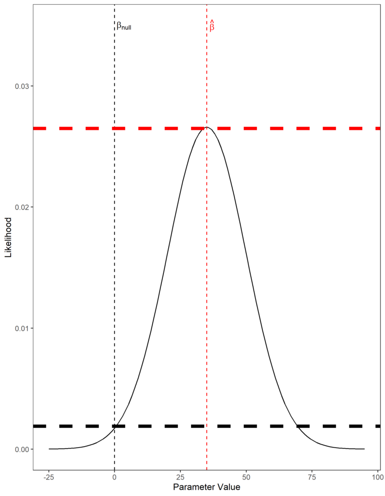
As in the Wald test, $Q_{LRT}$ follows asymptotically a $\chi^2$ distribution with 1 degree of freedom. This is ensured by multiplying the ratio by -2 - a mathematical proof exists to show that this test statistic does indeed follow this sampling distribution (derived here).

Note one major difference between this test and the Wald test is that we need to know $L(\beta_{null})$. This means that we need to actually fit the a model for the null hypothesis to obtain a likelihood. In the Wald test, we could get away with just knowing the expected value of $\beta_{null}$ - a value we have chosen and that does not need to be estimated from a model. With infinite sample sizes, both tests would converge on the same test statistics if the null hypothesis was true. However, the Wald test does not perform as well on small sample sizes than the LRT. Thus, the choice between a LRT and a Wald test depends on what is most appropriate for the data being analysed. If the data are huge, and the computational cost of fitting multiple models is large, a Wald test, or the score test (discussed next), may be preferred.

Score (Lagrange Multiplier) Test

The score test, also known as the Lagrange multiplier test, only requires the one model to be fit as is the case with the Wald test. Rather than use ratios between likelihoods, or differences between parameter estimates, the score test uses the gradient of the log likelihood function at the value of $\beta_{null}$, also known as the score at $\beta_{null}$, written as $S(\beta_{null})$:

$$ \begin{equation} Q_{score} = \frac{S(\beta_{null})^2}{I(\beta_{null})^{-1}} \end{equation} $$ $$ \begin{equation} S(\beta_{null}) = \frac{dlogL(\beta_{null})}{\beta_{null}} \end{equation} $$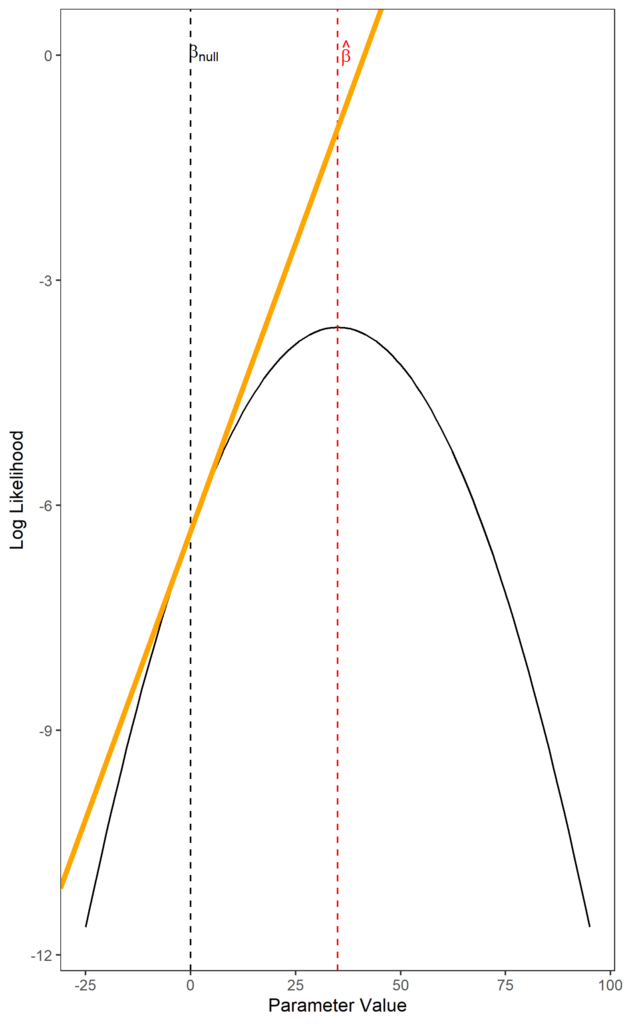

Tangent line at the parameter value under the null hypothesis shown in orange. The slope of this line is the score. Observe how the slope becomes steeper the further away from the MLE you move.

The gradient of the log likelihood at $\hat{\beta}$ is 0, because this is the maxima of the log likelihood function. We assume that the higher the score of $\beta_{null}$, the further away it is from the maximum likelihood estimate. Thus, the test statistic is higher, reflecting that $\hat{\beta}$ is unlikely to equal $\beta_{null}$. $Q_{score}$ follows asymptotically a $\chi^2$ distribution with 1 degree of freedom (proof here).

This value is divided by the Fisher information for $\beta_{null}$. Recall that for the Wald test, $var(\hat{\beta})$ is given by the inverted second derivative of the log likelihood function at the MLE, also known as the inverted Fisher information $I(\hat{\beta})^{-1}$. The Fisher information, $I(\hat{\beta})$, is actually an estimate of the variance of a score (if you’re interested in more details why, look up the Cramér–Rao bound). The more variable the score, the higher the Fisher information, and vice versa.

If we performed our sheep experiment many times, each time we would get a slightly different value of $S(\beta_{null})$ because of sampling error, even though $\beta_{null}$ doesn’t change. Therefore, $S(\beta_{null})$ has a variance, and this variance is estimated by $I(\beta_{null})$. If this variance is large, our estimate of the score is less certain, so we should be less confident in declaring that a large score means the true value of $\beta$ is far from $\beta_{null}$. Hence the division by the Fisher information.

The score test, Wald test, and LRT will all converge on the same test statistic as sample sizes grow, if the null hypothesis is true. The score test, much like the Wald test, does not perform as well as LRT on small sample sizes. However, you only have to fit a single model: the null model. Contrast this to the Wald test, where you only fit the alternative model. This property of the score test makes it a particularly good choice if you are testing lots of parameters simultaneously, and fitting the alternative model requires lots of computational resource.

A really accessible, but complete, and freely available introduction to likelihood-based hypothesis testing is Induction! An interactive introduction.