TidyTuesday: Oregon Spotted Frogs
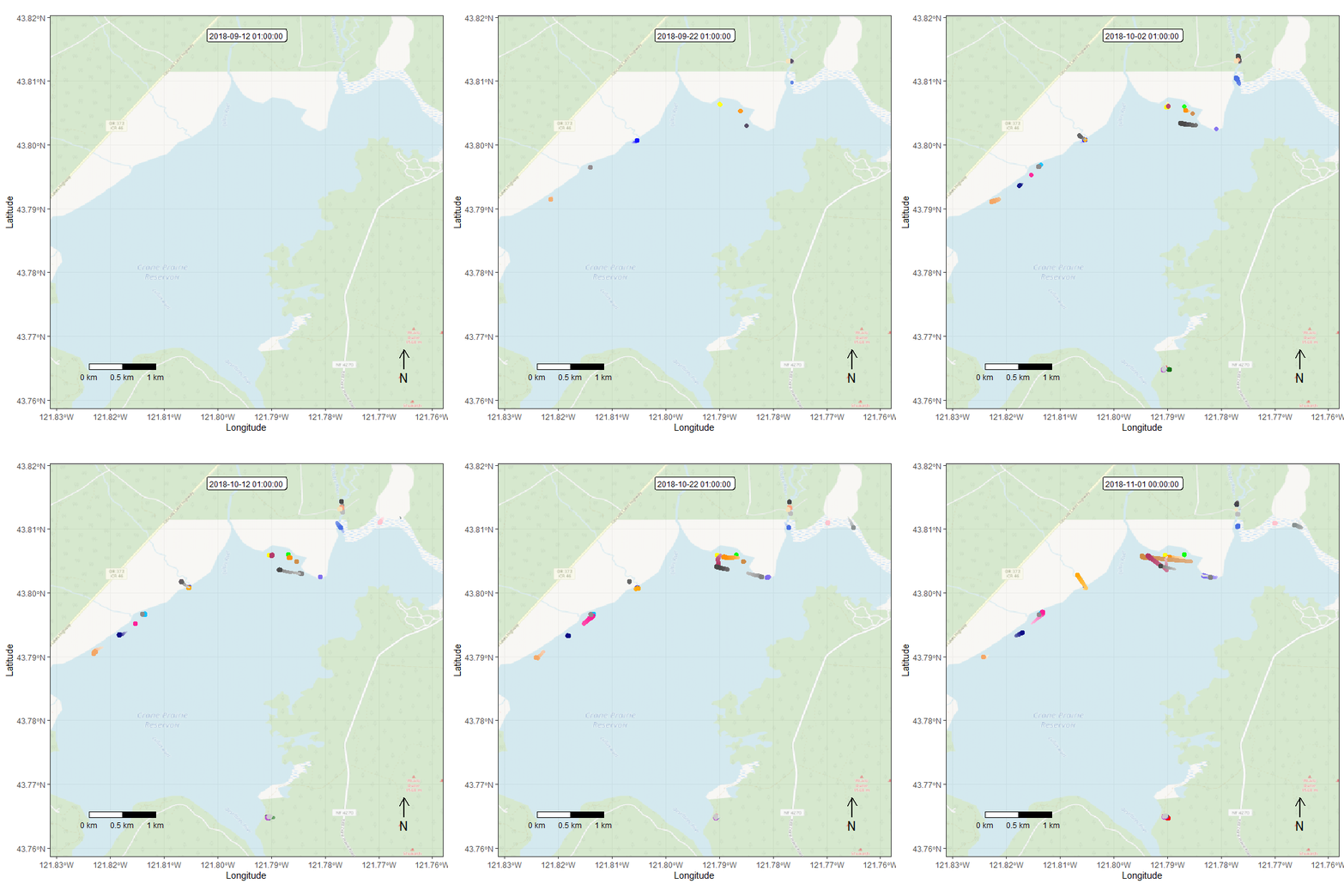
Frogs! I always have to show up for an animal themed week. Unfortunately, Oregon spotted frog numbers are in decline. This motivated the United States Geological Survey (USGS) to undertake a tracking study of Oregon spotted frogs in the Crane Prairie Reservoir. The locations of frogs was recorded roughly once a week for 10 weeks in 2018. For this data visualisation challenge, I create an animation of individual frog’s movements over this short period.

Each point on the graph represents an individual frog. The date of the recording is shown in a box at the centre top of the graph. The movement of frogs represents their actual movement over time.
This choice of animated visualisation in this scenario has the advantage of showing the viewer both the distribution of observed frogs and the movement of the frogs over time.
To make this vis, I used the moveVis package. This package is used to visualise movement through space over time. For example, to visualise the movement of GPS tracked animals, just as I did here! The other packages and data used to create this vis were:
library(moveVis)
library(lubridate)
library(terra)
library(tidyverse)
tuesdata <- tidytuesdayR::tt_load('2022-08-02')
The data came with Universal Transverse Mercator (UTM) Eastings and Northings. I transformed these into World Geodetic System (WGS) 84 longitude and latitudes using the project function from the terra R package.
utm_coords <- tuesdata$frogs[,c("UTME_83", "UTMN_83")]
utm_coords <- as.matrix(rename(utm_coords, "x" = "UTME_83", "y" = "UTMN_83"))
utm_coords <- vect(utm_coords, crs="+proj=utm +zone=10T +datum=WGS84  +units=m")

long_lat <- project(utm_coords, "+proj=longlat +datum=WGS84")
Then, using these longitudes and latitudes, a MoveStack object can be constructed using these co-ordinates and other data from the original frogs data: SurveyDate (when the frog was observed) and Frequency (this is the radio frequency used to track each frog, thus identifies individual frogs). MoveStack objects are the required input data type for creating a gif with moveVis.
long_lat <- geom(long_lat)[, c("x", "y")]

frogs <- cbind(long_lat, tuesdata$frogs)

frog_moves <- df2move(frogs,
        proj = CRS("+proj=longlat +datum=WGS84"),
        x = "x",
        y = "y",
        time = "SurveyDate",
        track_id = "Frequency")
Next, we need to set the time points that should be used for the gif. The data here is quite sparse, each frog only has a small number of recordings. So I chose one data point per day.
frog_moves <- align_move(frog_moves,
                         res = 1,
                         unit = "days")
Then, some magic from the moveVis package brings the animation to life. frames_spatial() creates each of the individual graphs that make up the gif, then animate_frames() makes these into a gif.
frames <- frames_spatial(frog_moves,
                         map_service = "osm",
                         alpha = 0.5,
                         path_legend = FALSE) %>%
  add_labels(x = "Longitude", y = "Latitude") %>%
  add_northarrow() %>%
  add_scalebar() %>%
  add_timestamps(frog_moves, type = "label") %>%
  add_progress()

animate_frames(frames, out_file = "frogmovements.gif")
And ta-da! An animated gif of Oregon spotted frog movements.